Category Archives: CFD

Comsol is Great

Definitely one of my favorite CAE programs is Comsol. I will tell you why. But first, some background. I have used a lot of CAE software, to make a short list:

  • agros2d
  • Comsol/Femlab
  • CalculiX
  • Elmer
  • Z88
  • Autodesk Simulation (formerly Algor)
  • ANSYS
  • Solidworks Simulation (CosmosWorks)
  • NX CAE, Nastran, Flow, etc.
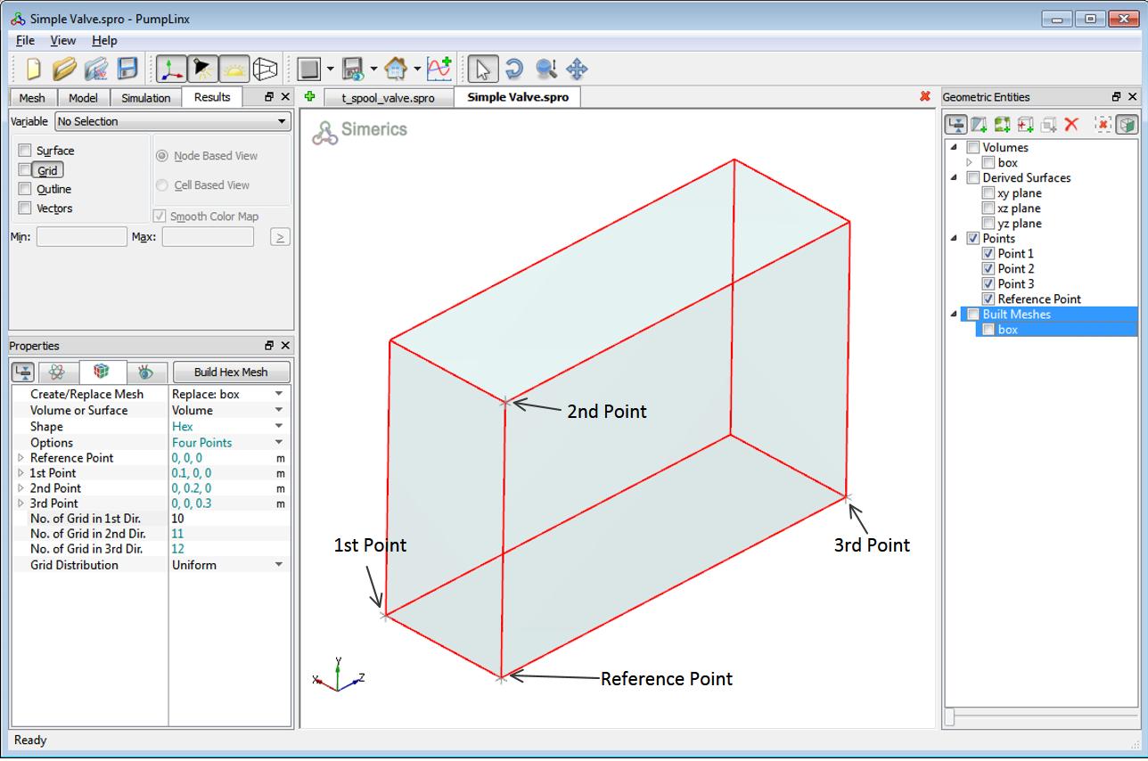
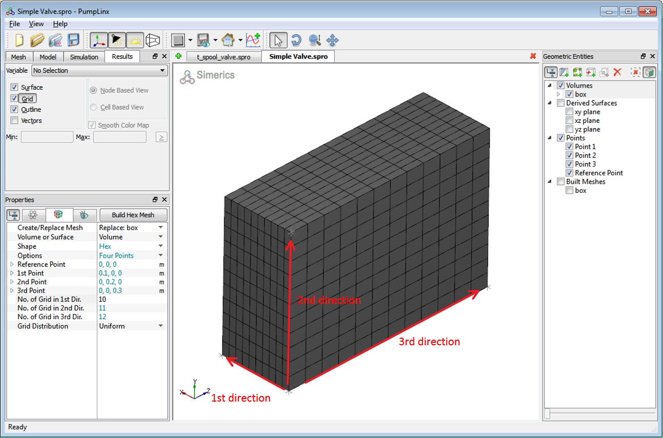
  • Simerics Pumplinx
  • Code_Aster
  • Salome
  • OpenFoam

I am a power user of CAE. I have done a lot and thus seen a lot FEA and CFD. I am also a fan so I read up on the latest techniques such XFEM for crack propagation.

So, in looking at many different platforms, I can say that COMSOL is a very rich and modern platform. Every place you enter information, you can enter an expression. This is important because almost anything can be linked or made dependent on something else. For example, a viscosity that is locally pressure and temperature dependent can be implemented based a 2d lookup table in COMSOL. Another example is solving simple contact problems. Contact is where the loads are displacement dependent. Thus, if you can define the function that defines the force or pressure between two surfaces as a function of position, then you can solve a contact problem without having to use a searching algorithm between surfaces. This is useful for simple problems and may not be so useful in complicated problems where defining the displacement dependent forcing function is difficult.

COMSOL is a much better program than ANSYS even though ANSYS is the industry defacto standard for FEA. COMSOL is easier to use and more modern in the interface and coupling of Multiphysics. The couple between different physics is done via modules or input your own PDE. While entering your own PDE sounds daunting, you don’t have to do that. You can just mix and match the modules using expression to couple material, boundary conditions, mesh, and other phenomenon to get the desire results.

Final comments: The COMSOL User interface is a thing of beauty. The documentation is outstanding.

Here is some screen shots from solving the Flow Past a cylinder example.

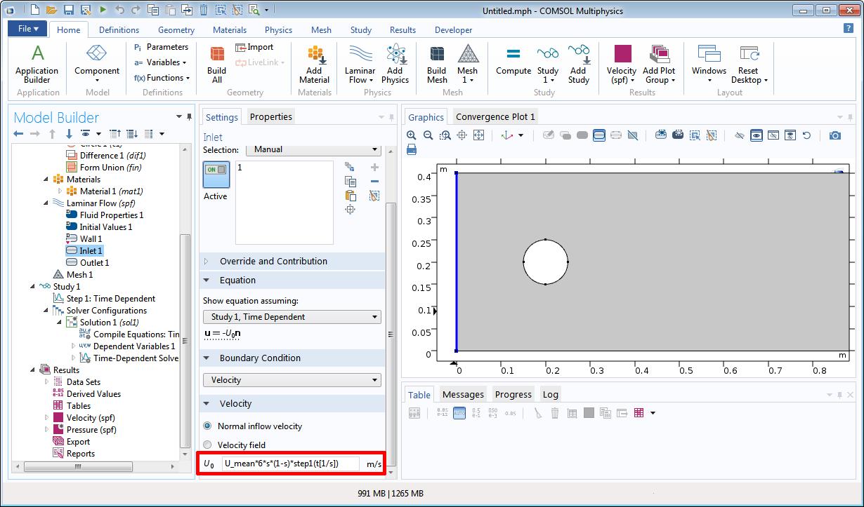
Example of a Comsol expression for a time dependent velocity.


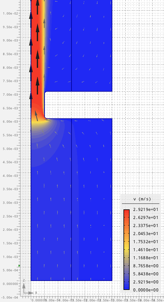
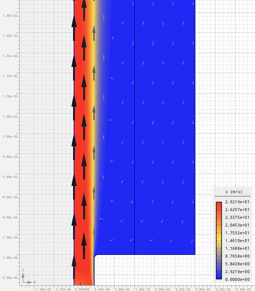
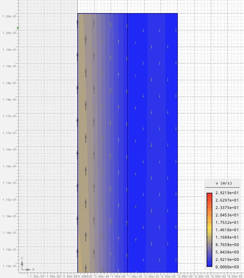
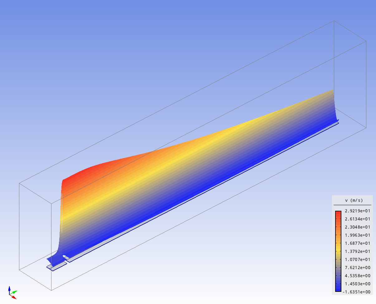
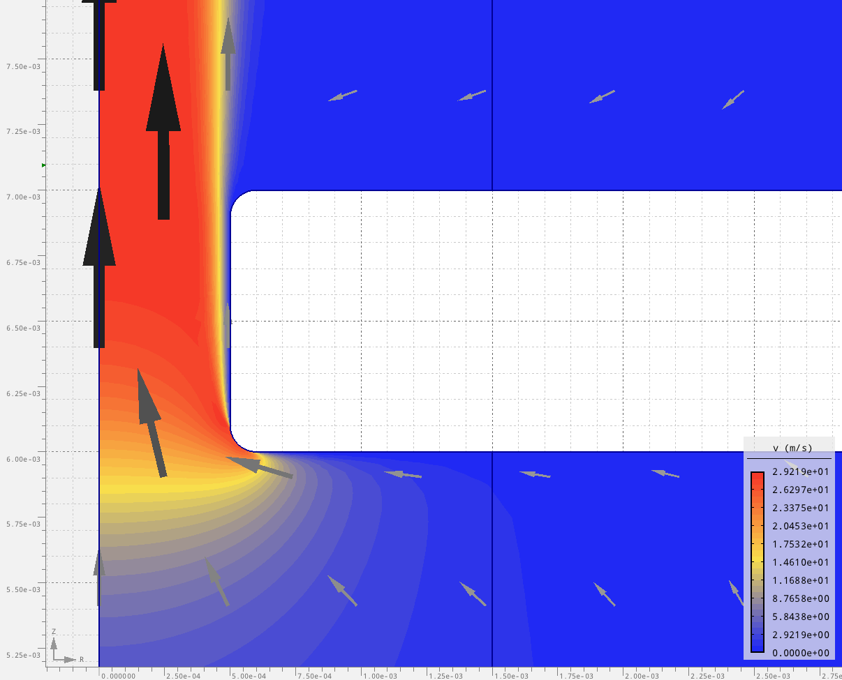
Velocity field in flow past a cylinder example.

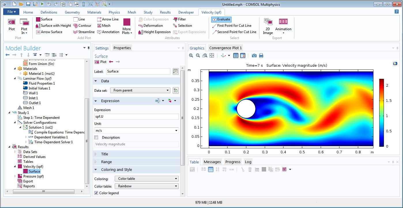
Velocity Field Past a Cylinder

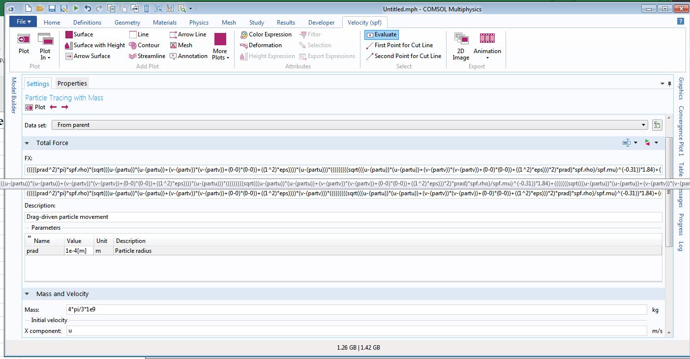
This one of the large expressions used for particle tracking in a fluid. See. It is an expression. A big one.

Simerics Pumplinx Hex Mesh Tutorial

Simerics Pumplinx sometimes doesn’t do a a good job in the help describing certain task such as Hex template meshing.  Here is some graphics that may help.


Layout of 4 point Hex Mesh in Simerics Pumplinx.


Mesh direction relationships. 1st direction points towards first point.
2nd direction point. etc.


Here are the files: Hex Mesh.zip

My Introduction to Computational Fluid Dynamics (CFD)

I have been doing a lot of CFD lately. I have quickly learned that the information one can gain from CFD is far more insightful to the physicals then 0D, lumped parameter equations.

One tool I have been using is Agros2d. It can do 2d axis symmetric and planar PDE problems. Agros2d can handle incompressible steady and unsteady CFD.

As an example, orifice problem has been studied many times. However, it usually isn’t studied from the point of view of an axis symmetric CFD.

Here is the model:Screenshot from 2016-05-07 00:50:44

The inlet boundary condition is a max velocity of 1.5m/s with a parabolic profile (1-(r/R)^2)*1.5m/s. R is the radius of the pipe 0.003m.

The Agros2d model is attached here: Orifice.a2d. You should be able to open the model with Agros2d and hit the “Solve” button in the lower left hand corner.

Below are some the results from the simulation.

Plot01

Velocity field near the beginning and throat.

Plot02

Velocity field just past the throat. Notice the re-circulation.

Velocity field at the outlet. Notice the recirculation

Velocity field at the outlet. Notice the recirculation

.

Velocity along the axis of the pipe (velocity in the z direction).

Velocity along the axis of the pipe (velocity in the z direction).

Velocity color plot at the throat. Notice that there is a dead space between the wall and the stream. The thinniest part of the stream is known as the vena contracta. See the next picture to see the velocity profile across the center of the throat.

Velocity color plot at the throat. Notice that there is a dead space between the wall and the stream. The thinnest part of the stream is known as the vena contracta. See the next picture to see the velocity profile across the center of the throat.

Plot07

This the velocity profile at the center of the throat. It is interesting to see the velocity is in a step shape. The velocity is constant in the stream and near zero otherwise.

Velocity profile at the start of throat where the fluid is accelerating.

Velocity profile at the start of throat where the fluid is accelerating.

Velocity profile at the end of the throat.

Velocity profile at the end of the throat.

Velocity profile at the outlet in the z direction which along the axis of the pipe. Notice the negative velocity part of the profile indicating recirculation.

Velocity profile at the outlet in the z direction which along the axis of the pipe. Notice the negative velocity part of the profile indicating recirculation.

Hopefully you enjoyed this as much as I did making it.