Trust-Region-Dogleg and Newton-Raphson – A Quick Comparison on a 5th order polynomial

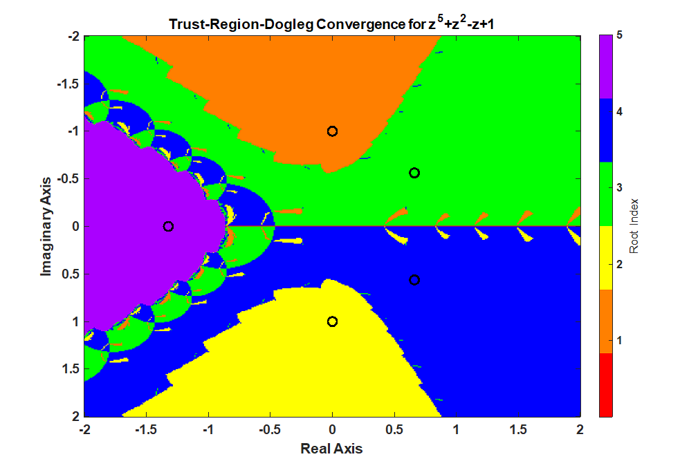
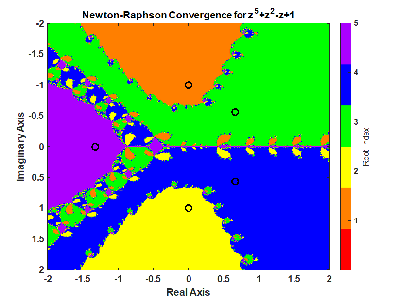
A Newton-Raphson iteration produces a fractal pattern in the complex plane and a Trust-Region-Dogleg method produces a smoother pattern in the complex which is desirable for a nonlinear equation solver. The context of this statement is finding the roots of a polynomial in a complex plan from different starting points. The inspiration for this post was the video from 3Blue1Brown, Newton’s Fractal (which Newton knew nothing about).

    clc;clear; close all;

Given the polynomial

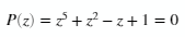
find a root starting from anywhere in the interval of -2 to 2 and -2i to 2i.

common code

% setup polynomial function
coefficients = [1 0 0 1 -1 1];
polynomialFunction = @(z) polyval(coefficients, z);
 
% setup the derivative of the polynomial function
coefficients_dot = polyder(coefficients);
polynomialDerivativeFunction = @(z) polyval(coefficients_dot, z);
 
% roots of the polynomial. roots uses a eigenvalues of a companion matrix approach.
% rootsOfPolynomial = roots(coefficients);
 
% exact roots
rootsOfPolynomial(1) = -1i;
rootsOfPolynomial(2) =  1i;
rootsOfPolynomial(3) =  (2^(2/3)*(3^(1/3) - 3^(5/6)*1i)*(69^(1/2) + 9)^(1/3))/12 + (2^(2/3)*3^(1/3)*(9 - 69^(1/2))^(1/3))/12 + (2^(2/3)*3^(5/6)*(9 - 69^(1/2))^(1/3)*1i)/12;
rootsOfPolynomial(4) =  (2^(2/3)*(3^(1/3) + 3^(5/6)*1i)*(69^(1/2) + 9)^(1/3))/12 + (2^(2/3)*3^(1/3)*(9 - 69^(1/2))^(1/3))/12 - (2^(2/3)*3^(5/6)*(9 - 69^(1/2))^(1/3)*1i)/12;
rootsOfPolynomial(5) = -(2^(2/3)*3^(1/3)*((69^(1/2) + 9)^(1/3) + (9 - 69^(1/2))^(1/3)))/6;
 
 
% Calculate a grid of starting points using the ndgrid format. x (real part)
% follow rows (1st dimension) and y follows the columns (2nd dimension).
% ndgrid is format is transpose of meshgrid format. meshgrid format is used
% for plotting surfaces.
nStartingPointReal = 400;
nStartingPointImaginary = 401;
startingPointReal = linspace(-2,2,nStartingPointReal)';
startingPointImaginary = linspace(-2,2+eps(2),nStartingPointImaginary)*1i;
startingPoint = startingPointReal + startingPointImaginary; % using singleton expansion
 
maxIterations = 100;
functionTolerance = 1e-14;
divideByZeroTolerance = 1000; % 1000*eps(p)

Newton-Raphson Iteration

Using Newton’s method starting anywhere in the interval -2 to 2 and -2i to 2i produces the following pattern.

% setup for iteration
isConverged = false(nStartingPointReal, nStartingPointImaginary);
isDivideByZero = false(nStartingPointReal, nStartingPointImaginary);
 
whileFlag = true;
iteration = 0;
z = startingPoint;
 
% check if the starting value was already converged.
% polynomial is less then functionTolerance.
p = polynomialFunction(z(~isConverged));
isConverged(~isConverged) = abs(p) < functionTolerance;
 
% begin iteration
p = polynomialFunction(z(~isConverged));
while whileFlag
    % increment iteration number
    iteration = iteration + 1;
 
    p = polynomialFunction(z(~isConverged));
 
    % Calculate the derivative of the polynomial.
    % Check for divide by 0. If p_dot is close to machine precision
    % of p, then its a divide by 0 error. 
    % Stop all further iteration.
    p_dot = polynomialDerivativeFunction(z(~isConverged));
    isDivideByZeroIteration = abs(p_dot) < divideByZeroTolerance*eps(abs(p));
    isDivideByZero(~isConverged) = isDivideByZeroIteration;
    isConverged(~isConverged) = isDivideByZeroIteration;
 
    % calculate Newton iteration on unconverged points.
    z(~isConverged) = z(~isConverged) - p(~isDivideByZeroIteration)./p_dot(~isDivideByZeroIteration);
 
    % check for convergence
    p = polynomialFunction(z(~isConverged));
    isConverged(~isConverged) = abs(p) < functionTolerance;
 
    % set while flag
    % all roots have converged or reached max iterations
    whileFlag = iteration <= maxIterations || all(all(~isConverged));
end
 
% successful roots
isRoot = isConverged & ~isDivideByZero;
 
% which root did newton's method converge too?
% calculate the difference between the converged root and the roots of the polynomial
% the smallest distance corresponds to the root index
zDiff = abs(z - reshape(rootsOfPolynomial,1,1,[])); % using singelton expansion
[rootErrors,rootIndex] = min(zDiff,[],3); % minimum along 3rd dimension
rootIndex(~isRoot) = 0;
 
% create the fractal image
% imagesc uses the meshgrid format where 
% x is the 2nd dimension 
% y is the first dimension
% therefore, transpose rootIndex because its in the ndgrid format
figure;
imagesc(startingPointReal', imag(startingPointImaginary), rootIndex')
c = prism(numel(rootsOfPolynomial)+1);
colormap(c);
xlabel("Real Axis"); ylabel("Imaginary Axis")
ylabel(colorbar('Ticks',1:numel(rootsOfPolynomial)),"Root Index")
hold all;
plot(rootsOfPolynomial,'ko','MarkerSize',10,'LineWidth',3)
title("Newton-Raphson Convergence for z^5+z^2-z+1")
Red is unconverged. The other colors correspond to a root. The o’s are the roots.

Trust-Region-Dogleg Iteration

The MATLAB fsolve() function uses the Trust-Region-Dogleg method to find a root of a nonlinear equation. What’s interesting is how much smoother the boundaries are for the Trust-Region-Dogleg method.

More information on Trust-Region-Dogleg method
Powell’s dog leg method – Wikipedia
Trust-Region-Dogleg Algorithm – MathWorks

options = optimoptions('fsolve','Display',"none","SpecifyObjectiveGradient",true, ...
    'FunctionTolerance',functionTolerance, 'StepTolerance',max(rootErrors(isRoot)),...
    "Algorithm","trust-region-dogleg");
% calling fsolve with the first argument as a cell array is undocumented but it works and is easy to setup. In a future
% version of MATLAB, this may not work because its undocumented. Also, each root is found one at a time and this is 
% ver inefficient. This could be a lot better but that is not the focus of today.
% 
tic;
[z2,~,exitflag2] = arrayfun(@(z0) fsolve({polynomialFunction,polynomialDerivativeFunction},z0,options),startingPoint);
toc;

Elapsed time is 406.891834 seconds.

% successful roots
isRoot2 = exitflag2 == 1;
 
% which root did the Trust-Region-Dogleg method converge too?
% calculate the difference between the converged root and the roots of the polynomial
% the smallest distance corresponds to the root index
zDiff2 = abs(z2 - reshape(rootsOfPolynomial,1,1,[])); % using singelton expansion
[rootErrors2,rootIndex2] = min(zDiff2,[],3); % minimum along 3rd dimension
rootIndex2(~isRoot2) = 0;
 
% create the fractal image
% imagesc uses the meshgrid format where 
% x is the 2nd dimension 
% y is the first dimension
% therefore, transpose rootIndex2 because its in the ndgrid format
figure;
imagesc(startingPointReal', imag(startingPointImaginary), rootIndex2')
colormap(c);
xlabel("Real Axis"); ylabel("Imaginary Axis")
ylabel(colorbar('Ticks',1:numel(rootsOfPolynomial)),"Root Index")
hold all;
plot(rootsOfPolynomial,'ko','MarkerSize',10,'LineWidth',3)
title("Trust-Region-Dogleg Convergence for z^5+z^2-z+1")
Red is unconverged. The other colors correspond to a root. The o’s are the roots.

Neural Networks. Controls, and System Identification

The current engineer atmosphere is buzzing about Neural Networks. The downside is that Neural Networks do not have a structure that is easily understandable and interpretable. When we can understand the physic mechanisms, Neural Networks should not be your first choice, in my opinion.

The links below take you directly to the start of the pertinent question(s). Among the two controls authors, they agree we can do the same or better than Neural Networks. Gene Morelli is from NASA. Stephen Boyd is from Standford.

Gene Morelli from NASA responds about Neural Networks. The video jumps to the start of this question at 1:19:43, and the question is finished at 1:21:30. The total question time is 1:47.

Stephen Boyd Response to Neural Network Use in Optimization and Control Question starts at 1:40:48. It gets interesting at 1:43:15. The question concludes at 1:44:47. The total question time is 3:59.

The counterpoint to my viewpoint is Chris Rackauckas’s Automated Discovery of Mechanistic Models via Universal Differential Equations. Sometime in the future, Neural Networks may dominate. For now, I don’t see it this way and think controls engineers should use other methods if they can understand their system.

System Identification Resources

What is System Identification? System Identification Wikipedia

Books

Lennart, Ljung. “System identification: theory for the user.” PTR Prentice Hall, Upper Saddle River, NJ 28 (1999). Errata can be found here.

Juang, Jer-Nan. Applied system identification. Prentice-Hall, Inc., 1994.

Morelli, Eugene A., and Vladislav Klein. Aircraft system identification: theory and practice. Vol. 2. Williamsburg, VA: Sunflyte Enterprises, 2016.

Soderstrom and P. Stoica, System Identification, Prentice Hall. 1989 (available for download from the author’s website)

Brunton, Steven L., and J. Nathan Kutz. Data-driven science and engineering: Machine learning, dynamical systems, and control. Cambridge University Press, 2022. Available here: https://www.databookuw.com/

I have created a list of system identification books via WorldCat. WorldCat allows you to search libraries across the wold. WorldCat Book List.

Researchers

Google Scholar search by System Identification label.

Online Course

System Identification by Roy Stephen Smith from ETH Zürich. Video lectures only. At the time of writing this, a course webpage that is more current than the lectures can be found here.

System Identification and Parameter Estimation from TUDelft OpenCourseWare. Has videos.

System Identification at Linköping University. Not an online course but gives a recommended schedule of lectures and readings. To preserve this information for the future, a screenshot is below of the schedule.

Lecture notes and recordings for ECE5560: System Identification. Uses Lennart Ljung’s book.

System Identification IIT Madras, Prof. Dr. Arun K.Tangirala. Video lectures are available.

System Identification via MIT OpenCourseWare – This course uses Lennart Ljung’s Book. No videos. A syllabus (outline), calendar, lecture notes, and assignments are available.

System identification: parametric approach an approximate 27-hour (English) lecture series on system identification using parametric approaches. See the selected topics and handouts at http://jitkomut.eng.chula.ac.th/ee531… Instructor: Jitkomut Songsiri, Chulalongkorn University, Thailand

Identification, Estimation, and Learning MIT 2.160
2.160 Identification, Estimation, and Learning Youtube
2.160 Identification, Estimation, and Learning Panopto Video
https://darbelofflab.mit.edu/teaching/ Slides and Notes can be obtained from links on this page.

Videos

Technical Seminar: ‘Quest for Aircraft Stability and Control’ by Eugene Morelli. Testing of full-scale aircraft in flight to validate or improve predictions obtained through wind tunnel testing or CFD calculations is expensive and time-consuming. Being able to test aircraft stability and control using real-time onboard computations is now within reach and has far-reaching implications for efficient flight testing, control system design, aircraft health monitoring, pilot training, aircraft fleet maintenance, and safety. Aired May 18, 2007.

Introduction to System Identification. An introduction to System Identification with the System Identification Toolbox in MATLAB. Lennart Ljung is the presenter.

Linear system identification video lecture – YouTube playlist. The video course “System identification – linear theory” introduces the student to linear system identification techniques based on data-driven modeling techniques. The focus lies on experiment design, understanding and selecting model structures, and computing the best model within the model set using prediction error methods and model validation.

System Identification. Videos by Brian Douglas. Throughout the series, see the system identification workflow through several different examples that highlight the importance of data collection, model selection, model fitting, and model validation in MATLAB with the System Identification Toolbox.

Software

MathWorks System Identification Toolbox This one is written by Lenart Ljung at least initially. His book is linked above. Uses Lennart Ljung’s book.

System/Observer/Controller Identification Toolbox (SOCIT) This one is written at least initially by Jer-Nan Juang; his book is linked above. This is free but export-controlled.
SOCIT is a collection of functions, written in MATLAB language and expressed in M-files, that implements a variety of modern system identification techniques. For an open-loop system, it features functions for identification of a system model and corresponding forward and backward observers directly from input and output data. For a closed-loop system, SOCIT identifies an open-loop model, an observer, and a corresponding controller gained directly from input and output data.

System IDentification Programs for AirCraft (SIDPAC) This one is written and maintained by Gene Morelli. His book is linked above. It is free and allowed for foreign use (not export controlled).
Written in MATLAB, SIDPAC is a collection of over 300 programs that perform a wide variety of tasks related to system identification applied to aircraft. SIDPAC includes tools for experiment design, data analysis, kinematic consistency checking, static and dynamic modeling, simulation, numerical integration and differentiation, smoothing, filtering, finite Fourier transformation, statistical modeling and evaluation, optimization, parameter estimation, model accuracy quantification, model validation, and more.

Github Repositories

Mataveid System identification toolbox for GNU Octave and MATLAB was written by Daniel Mårtensson. It is mostly based on Applied System Identification.

More to come here….

Links

Database for the Identification of Systems (DaISy)

TEACHING SYSTEM IDENTIFICATION. GOALS AND FORMATS FOR DIFFERENT COURSES. Paper by Lennart Ljung

SSH, Windows, Web Servers, Linux, and Visual Studio Code

Introduction

The hardest thing about trying to do something new with computers these days is that it is hard to focus on the one new thing I am trying to learn. I want to start working on setting up a web server to implement engineering calculations at openhydrualics.com because I want them to be open and easy for anyone to use. This post is the saga I have been through to get to where I am today, a working web server that I can access to create the website I want.

Background

I volunteer on an ISO, International Organization for Standardization, committee writing a new standard for calculating derived displacement for the hydraulics industry. As I have listened to what is going on in the tech world, I have seen things like Alliance for Open Media (AOM). AOM has united businesses in collaboration to develop the next generation of video codecs called AV1. I want to do similar things in the hydraulics industry to save money and time, and move the world forward. It is a great way to impact the world, and it is my part in making the world we live in a better place. Therefore, I thought that building a unified implementation of hydraulic engineering calculations that are open source and delivered via the web is a great way to tie all of this together. This may end up being a non-profit, or it may just be an open-source project. We will see, and I am still exploring this. The real point today is getting the environment set up so that I can develop a web application.

The Saga

The first thing I had to decide was what programming language and toolset I would use to develop my web app. I know MATLAB really well. I would love to use MATLAB. To quote MATLAB help related to web apps:

[MATLAB] web apps are designed to run only within a trusted intranet environment, not in the open Internet. For more information, see Potential Risks.

https://www.mathworks.com/help/compiler/web-apps.html

So this looked like a nonstarter using MATLAB. Besides, was I going to pay for using MATLAB plus several toolboxes? Maybe. MATLAB is about $2000, with each toolbox costing another $2000. That isn’t too bad if all I had to pay was $4000-5000 plus a few days; this would be time-efficient. However, it isn’t a real option.

I started exploring other web apps such as Google Colab, Streamlit (Python), Genie (Julia), and Blockpad. Google Colab isn’t right because it requires sign-in and knowledge to use a Jupyter notebook with Python for my users. Blockpad is interesting but too basic for what I need; i.e., I need linear algebra and scientific computing. The Julia language was built for scientific computing. Genie was built to create web apps and looks good. Streamlit looks really good too. I want to learn Julia more than I want to learn Python because I tend to write scientific computing programs. As I have explored Genie and Julia, I am more sold that it is a good general direction.

Hosting was the next thing to consider. My website, jasonhnicholson.com, is hosted on Bluehost shared hosting. I learned that shared hosting is extremely locked down. I cannot use Julia or Python on the shared hosting platform in flexible enough ways. I had to compile python from scratch, which would have been fine if it worked, but it didn’t. It failed to compile correctly, which left me with a broken Python. I also tried Julia but received errors related to shared libraries (shown below), which told me that compiling was just a waste of time. I spent a whole weekend trying to solve the “Is shared hosting a good solution” question. I think shared hosting is not a good solution for running Julia or Python for my expertise level. It costs too much time.

user1@jasonhnicholson.com [~]# julia
julia: error while loading shared libraries: libjulia.so.1: cannot open shared object file: No such file or directory
user1@jasonhnicholson.com [~]#

Next up was I tried Virtual Private Server (VPS) for Bluehost, a step up compared to shared hosting. It gave access to a CentOS server with a package manager for around $30 a month; it could be cheaper, but I am paying monthly, so I don’t get it cheaper for a yearly subscription. Other services are cheaper, but I have used Bluehost for a while. Time is worth more than learning another hosting platform. Long term, I may do something different.

VPS was easier to work with than shared hosting. The downside was that it took a whole four days to get things working correctly between SSH, CPanel, WHM, Julia, yum, rpm, CentOS, Julia, bash, and more. If some of these things are not familiar to you, it should explain the vast difficulty of trying to work cross-disciplinary on the web. It isn’t easy. I am comfortable enough with Linux that bash doesn’t scare me. I google things just like everyone else. I can learn but be more focused when I can help it.

The Cpanel is a web hosting control panel. WHM is a Web Host Manager. Together Cpanel and WHM work to provide a web interface to my Bluehost VPS server. These were failing on the first setup to Bluehost. I ran into an infinite refresh of the Cpanel page. I started the VPS setup on a Friday. Six calls to Bluehost, and four days later, I had a working VPS server on Tuesday morning. My time is limited when I work on projects like this. I have maybe a few hours a weekend and nights. Having patience is important but a difficult discipline. Here was another lesson in patience and flexibility. I learned. I grew.

Next was SSH. SSH keys and SSH on windows don’t play well together. This where I have to understand Linux file permissions, SSH file requirements, Windows file permissions, and the different implementations of SSH across Linux and Windows. It’s a mess. The short story is to find the Microsoft OpenSSH repository. Putty works. Mosh works and is unusable. Git Bash works and is usable. However, I had to face the SSH file permissions concerning SSH keys on windows at some point. Microsoft has written Powershell scripts to deal with SSH key file permissions in the repo documentation: OpenSSH utility scripts fix file permissions. When I find the right information, it is amazing how simple this is to solve. When you don’t understand the problem and can’t find the right information, it is amazing the amount of time that can be wasted fighting this; I think it took me 5 days to understand the working parts of SSH, Linux, and Windows to finally solve this before I found the link to Microsoft OpenSSH repo. At least now I understand what is going on. I understand how to use ssh-agent to add my private key. I don’t use a private key without a password. My private key is heavily protected, and I think I know what I am doing around SSH now.

Visual Studio Code (VSCode) was next. Technically, it was mixed into SSH, but we don’t have to get into that. Visual Studio Code is a great tool, but it is another thing to learn. It has a lot of working parts. It is a good editor with lots of functionality, including a Julia IDE with Remote SSH extension ( screenshot below). VSCode has around 120 keyboard shortcuts to learn. If you are going to use an IDE a lot, learn the shortcut keys. I decided to learn VSCode by learning the shortcut keys, so I made a Quizlet of all the shortcut keys here: Visual Studio Code Keyboard Shortcuts Quizlet.

Visual Studio Code SSH session to my server and Julia

The Julia language, Genie.jl package, and the Stipple.jl package was next. Julia is an up-and-coming scientific computing language. All around, it seems that it is a good computer science language. I have been using Julia Documentation, Julia|Exercism, Julia REPL Shortcut Keys, Key bindings Quizlet (I created this), Julia Visual Studio Code Shortcut Keys, and the Julia Discourse. Exercism.com teaches through code by problem/challenge, which works well for me. Exercism allows me to look at other people’s solutions once I have submitted a solution. This is working for learning the Julia language. I am enjoying it. Quizlet is a great tool for memorizing lists. Julia Discourse is a great place to ask for help.

I will hire someone in the Julia community to mentor me and help with general direction concerning my web app. I need help and am willing to give up the money to save time. Web development isn’t my forte, but I can learn. I prefer to stay focused as much as I can.

Object-Oriented Programming Decline – The Rise of other Paradigms

I listen to a lot of computer science-related talks and podcasts. Recently, I have seen a trend away from the object-oriented paradigm. The premise is fusing your data and functions together is hard to maintain at scale. I agree. A better approach is only loosely to tie your data to the functions. I see this in the Julia language, for instance.

I watched several videos that led me to gather a little information on the issues. The first one was Why Isn’t Functional Programming the Norm? – Richard Feldman. He talks about why object-oriented programming came to be the norm in the ’90s and 2000s. The main reason he describes is Java. There is more to, but there isn’t a strong reason why the industry embraced object-oriented programming.

Next, the following video showed up in my YouTube feed: Object-Oriented Programming is Bad. The title is severe, and the content is less severe. The main issue comes back to that fusing your data and methods together doesn’t scale well.

Lastly, I watched JuliaCon 2019 | The Unreasonable Effectiveness of Multiple Dispatch | Stefan Karpinski as I explore the Julia language. The Julia Language focuses on generic programming, which is amazing that the same code can be used for different data. Generic programming generally requires splitting the data out from the algorithm, which goes against object-oriented programming.

Using the Shortname

The Shortname is a Windows way of dealing with non-ASCII characters and long file names and paths.

First, let’s create some filenames with bad character inside bad folder names. We will use the character map to generate some commonly used Unicode, non-ASCII characters. We will even use some Arabic characters. See Table 1. Note, that the files with long names longer than 260 characters require special care to generate and is not something a user can do easily. Figure 2 shows the error message windows give you when you try to create a file/path name that is too long.

Figure 1: Windows Character map showing what character sets windows supports.

Table 1: Shows the files with non-ASCII characters and long file paths along with their shortname.

File #Long NameLong Name LengthShort NameComments
1C:\Temp\example long file name with non ASCII character 1 - °±ØøθΘﮆﯶﯙ.txt73C:\Temp\EXAMPL~1.TXT
2C:\Temp\Long Folder Name with non ASCII characters 1 - °±ØøθΘﮆﯶﯙ\example long file name with non ASCII character 2 - °±ØøθΘﮆﯶﯙ.txt130C:\Temp\LONGFO~1\EXAMPL~1.TXT
3C:\Temp\Long Folder Name with non ASCII characters 1 - °±ØøθΘﮆﯶﯙ\example long file name with non ASCII character 3 - °±ØøθΘﮆﯶﯙ.txt130C:\Temp\LONGFO~1\EXAMPL~2.TXT
4C:\Temp\Long Folder Name with non ASCII characters 1 - °±ØøθΘﮆﯶﯙ\Long Folder Name with non ASCII characters 2 - °±ØøθΘﮆﯶﯙ\example long file name with non ASCII character 4 - °±ØøθΘﮆﯶﯙ - Copy.txt194C:\Temp\LONGFO~1\LONGFO~1\EXAMPL~2.TXT
5C:\Temp\Long Folder Name with non ASCII characters 1 - °±ØøθΘﮆﯶﯙ\Long Folder Name with non ASCII characters 2 - °±ØøθΘﮆﯶﯙ\example long file name with non ASCII character 4 - °±ØøθΘﮆﯶﯙ.txt187C:\Temp\LONGFO~1\LONGFO~1\EXAMPL~1.TXT
6C:\Temp\Long Folder Name with non ASCII characters 1 - °±ØøθΘﮆﯶﯙ\Long Folder Name with non ASCII characters 2 - °±ØøθΘﮆﯶﯙ\Long Folder Name with non ASCII characters 3 - °±ØøθΘﮆﯶﯙ\example long file name with non ASCII character 5 - °±ØøθΘﮆﯶﯙ.txt244C:\Temp\LONGFO~1\LONGFO~1\LONGFO~1\EXAMPL~1.TXT
7C:\Temp\Long Folder Name with non ASCII characters 1 - °±ØøθΘﮆﯶﯙ\Long Folder Name with non ASCII characters 2 - °±ØøθΘﮆﯶﯙ\Long Folder Name with non ASCII characters 3 - °±ØøθΘﮆﯶﯙ\Long Folder Name with non ASCII characters 4 - °±ØøθΘﮆﯶﯙ\example long file name with non ASCII character 6 - °±ØøθΘﮆﯶﯙ.txt301C:\Temp\LONGFO~1\LONGFO~1\LONGFO~1\LONGFO~1\EXAMPL~1.TXTPaths longer than 260 characters are trouble. I don't understand when you can work with them and when you can't.
8C:\Temp\Long Folder Name with non ASCII characters 1 - °±ØøθΘﮆﯶﯙ\Long Folder Name with non ASCII characters 2 - °±ØøθΘﮆﯶﯙ\Long Folder Name with non ASCII characters 3 - °±ØøθΘﮆﯶﯙ\Long Folder Name with non ASCII characters 4 - °±ØøθΘﮆﯶﯙ\Long Folder Name with non ASCII characters 5 - °±ØøθΘﮆﯶﯙ\example long file name with non ASCII character 7 - °±ØøθΘﮆﯶﯙ.txt358C:\Temp\LONGFO~1\LONGFO~1\LONGFO~1\LONGFO~1\LONGFO~1\EXAMPL~1.TXTPaths longer than 260 characters are trouble. I don't understand when you can work with them and when you can't.
Figure 2: What happens when a path or file name is too long.

If you use the command “dir /s /b example*.txt” then you get the block of text shown in Block 1. Note that the dir did not return the 8th file path. This is because it has a local folder path longer than 260 characters.

C:\Temp\example long file name with non ASCII character 1 - °±ØøθΘﮆﯶﯙ.txt
C:\Temp\Long Folder Name with non ASCII characters 1 - °±ØøθΘﮆﯶﯙ\example long file name with non ASCII character 2 - °±ØøθΘﮆﯶﯙ.txt
C:\Temp\Long Folder Name with non ASCII characters 1 - °±ØøθΘﮆﯶﯙ\example long file name with non ASCII character 3 - °±ØøθΘﮆﯶﯙ.txt
C:\Temp\Long Folder Name with non ASCII characters 1 - °±ØøθΘﮆﯶﯙ\Long Folder Name with non ASCII characters 2 - °±ØøθΘﮆﯶﯙ\example long file name with non ASCII character 4 - °±ØøθΘﮆﯶﯙ - Copy.txt
C:\Temp\Long Folder Name with non ASCII characters 1 - °±ØøθΘﮆﯶﯙ\Long Folder Name with non ASCII characters 2 - °±ØøθΘﮆﯶﯙ\example long file name with non ASCII character 4 - °±ØøθΘﮆﯶﯙ.txt
C:\Temp\Long Folder Name with non ASCII characters 1 - °±ØøθΘﮆﯶﯙ\Long Folder Name with non ASCII characters 2 - °±ØøθΘﮆﯶﯙ\Long Folder Name with non ASCII characters 3 - °±ØøθΘﮆﯶﯙ\example long file name with non ASCII character 5 - °±ØøθΘﮆﯶﯙ.txt
C:\Temp\Long Folder Name with non ASCII characters 1 - °±ØøθΘﮆﯶﯙ\Long Folder Name with non ASCII characters 2 - °±ØøθΘﮆﯶﯙ\Long Folder Name with non ASCII characters 3 - °±ØøθΘﮆﯶﯙ\Long Folder Name with non ASCII characters 4 - °±ØøθΘﮆﯶﯙ\example long file name with non ASCII character 6 - °±ØøθΘﮆﯶﯙ.txt

Block 1

If instead we dump the command to a text file “dir /s /b example*.txt > filelist.txt” then we have a problem as shown in Block 2. Some of the non-ASCII characters become question mark characters. This makes working with these files just about unworkable through text files.

C:\Temp\example long file name with non ASCII character 1 - øñOo?é???.txt
C:\Temp\Long Folder Name with non ASCII characters 1 - øñOo?é???\example long file name with non ASCII character 2 - øñOo?é???.txt
C:\Temp\Long Folder Name with non ASCII characters 1 - øñOo?é???\example long file name with non ASCII character 3 - øñOo?é???.txt
C:\Temp\Long Folder Name with non ASCII characters 1 - øñOo?é???\Long Folder Name with non ASCII characters 2 - øñOo?é???\example long file name with non ASCII character 4 - øñOo?é??? - Copy.txt
C:\Temp\Long Folder Name with non ASCII characters 1 - øñOo?é???\Long Folder Name with non ASCII characters 2 - øñOo?é???\example long file name with non ASCII character 4 - øñOo?é???.txt
C:\Temp\Long Folder Name with non ASCII characters 1 - øñOo?é???\Long Folder Name with non ASCII characters 2 - øñOo?é???\Long Folder Name with non ASCII characters 3 - øñOo?é???\example long file name with non ASCII character 5 - øñOo?é???.txt
C:\Temp\Long Folder Name with non ASCII characters 1 - øñOo?é???\Long Folder Name with non ASCII characters 2 - øñOo?é???\Long Folder Name with non ASCII characters 3 - øñOo?é???\Long Folder Name with non ASCII characters 4 - øñOo?é???\example long file name with non ASCII character 6 - øñOo?é???.txt

Block 2

In VBA, the short name is not something that VBA functions are setup to work with. Instead, if you use the “del shortname” through a shell command, then you can delete the file(s). For instance executing the command in Block 3 deletes all 8 files from Table 1 and Block 4 shows that the files no longer exist, which includes the files with long paths. Since I did not obtain the long folder path of file 8 via dir, I am not sure how you would get its short name except for manually generating it.

del C:\Temp\EXAMPL~1.TXT C:\Temp\LONGFO~1\EXAMPL~1.TXT C:\Temp\LONGFO~1\EXAMPL~2.TXT C:\Temp\LONGFO~1\LONGFO~1\EXAMPL~2.TXT C:\Temp\LONGFO~1\LONGFO~1\EXAMPL~1.TXT C:\Temp\LONGFO~1\LONGFO~1\LONGFO~1\EXAMPL~1.TXT C:\Temp\LONGFO~1\LONGFO~1\LONGFO~1\LONGFO~1\EXAMPL~1.TXT C:\Temp\LONGFO~1\LONGFO~1\LONGFO~1\LONGFO~1\LONGFO~1\EXAMPL~1.TXT

Block 3

C:\Temp>dir /s /b  example*.txt
File Not Found

Block 4

FFmpeg, The -crf Option, iPhone Videos, and Corporate Networks

I use FFmpeg on a regular basis for video, audio, and image-related editing. It is a command-line tool that goes from very simple to very complicated. I intend to stick with simple today. The point here is you can save 80-90% of the space used by iPhone, GoPro, or Android Video by re-encoding the video with FFmpeg and the -crf option. Keep reading to learn more.

To use FFmpeg, use something like the following.

$ ffmpeg -i input.mp4 output.avi

The above code will convert an mp4 to an avi using inferred settings and won’t change the video’s codec. Side note, if you don’t know what a video format, container, and codecs are and how they relate, pause and read this link: Every Video Format, Codec, and Container Explained.

The problem I have run into is corporate network drives have lots of iPhone videos that have been stored for future reference. The first time I encountered this problem, I was working for ABC Company (to not name names or blame or whatever) and we ran out space on a network drive. We had several hundred engineers that could no longer work because we ran out space. IT could not expand the Network drive because of a limitation. This upset me. I couldn’t believe that this had happened at a large company and no one was doing anything about it. Therefore, I did something about it. I scanned the network to see what was stored on our network drive. The #1 space-consuming filetype was iPhone videos. People had dumped 300GB of iPhone videos onto our network over several years. Therefore I looked for a solution that could re-encode the videos, maintain the format, codec, resolution, framerate, and compatibility but reduce the file size. This is where FFmpeg and the -crf option comes in handy. All you have to do reduce the video size by 80-90% is the use the following code snippet

 ffmpeg -i inputMovie.mov -crf 28 outputVideo.mov

The above code snippet will maintain the format, codec, framerate, resolution, and then adjust the bitrate based on some factors documented better here: CRF Guide (Constant Rate Factor in x264, x265 and libvpx). I usually use a -crf of 28 for my x264 videos which is basically what all iPhone, GoPro, and Android videos are. This is aggressive but the loss of quality is minimal. For instance, a video that was 100MB will be 10MB after re-encoding it with -crf 28 and you can’t tell that I re-encoded the video.

The problem is that the bitrate of an iPhone video is an average of 20,000KB/s or more. Often, you don’t need that high of bitrate and it is overkill. After using -crf of 28, the bitrate will drop to an average of 2000KB/s or so. The bitrate during the video isn’t constant though. The bitrate is variable, you could have a segment of a video that is a bitrate of 10,000KB/s but still have an average 2000KB/s.

The 300GB’s of iPhone movies that I found on the ABC Company network, I re-encoded saving around 270GB. This allowed us to start working again on our Corporate Network drive.

Recently I was at XYZ Company, I did a check for videos on the network. We have 1400GB of videos on that Network drive. I am betting that we can save 1100GB by re-encoding the videos.